Preface

Recently, more and more works are published talking about pre-training strategies on molecular data, which lead to better performance on downstream tasks of molecules. However, the relationship between molecular representation and pre-training methods still remains a mystery. This blog is a brief note about two works taking about the evaluation of pre-training tasks on molecular data.

Note that the two works only talk about pre-training on 2D molecular data. For 3D molecular data, there might be different results with 2D data.

Does GNN Pretraining help molecular representation?

Description

In this paper, the author perform systematic studies to assess the performance of popular graph pretraining techniques on different types of molecular datasets, and exploit various confounding components in experimental setup in deciding the performance of downstream tasks with or without pretraining.

The author have evaluated the following pre-training tasks:

self-supervised pretraining:
- Node prediction (node-level task): some proportion of node attributes are masked and replaced with mask-specified indicators in the node input feature. After graph convolution, the embedding output from GNN is used to predict the true attribute of the node, e.g. atom type in molecular graphs, through a linear classifier on top of the node embedding.
- Context prediction (sub-graph level task): aiming at learning embedding that can represent the local subgraph surrounding a node
- Motif prediction (graph-level task): aiming at learning embedding that can represent the local subgraph surrounding a node. Graph embedding is used to jointly predict the occurrence of these semantic functional motifs.
- Contrastive learning: to maximize the agreement of two augmented views of the same graph, and minimize the agreement of different graphs. The optimization is conducted using contrastive loss in the latent embedding space. The augmentation function needs to transform graphs into realistic and novel augmentations without affecting semantic labels of the graphs.
supervised pretraining: aims to learn domain-specific graph-level knowledge from specific designed pretraining tasks.

Experiment design

self-supervised learning:
- masking: randomly masks 15% of the nodes’ feature
- context prediction: masks out the context from k1-hops to k2-hops and leverages adversarial training to predict the true context embeddings from the random context embeddings
- motif prediction: GNN is asked to predict whether a motif is contained in a molecule. The motif can be extracted from the molecule with RDKit.
- contrastive: corrupt the input node features with Gaussian noise to generate different views of the same graph, and maximize the consistency between positive pairs (same graph) and minimize that between negative pairs (different graphs).
- graph-level supervised: use the ChEMBL dataset with graph-level labels for graph- level supervised pretraining
graph features (mainly consider the graph representations without the 3D information):
- basic features: the node features contain the atom type and the derived features, such as formal charge list, chirality list, etc. The edge features contain the bond types and the bond directions.
- rich features (default): The rich feature set is a superset of the basic features. In addition to the basic ones mentioned above, it comes with the additional node features such as hydrogen acceptor match, acidic match and bond features such as ring information.
pretraining dataset: ZINC15(default), SAVI for SSL, ChEMBL for supervised.
GNN backbone: GIN(default), GraphSAGE
dataset split: scaffold Split — first sorts the molecules according to the scaffold (e.g. molecule structure), and then partition the sorted list into train/valid/test splits consecutively. And Balanced Scaffold Split (default) — introduces randomness in sorting and splitting stages.

Result

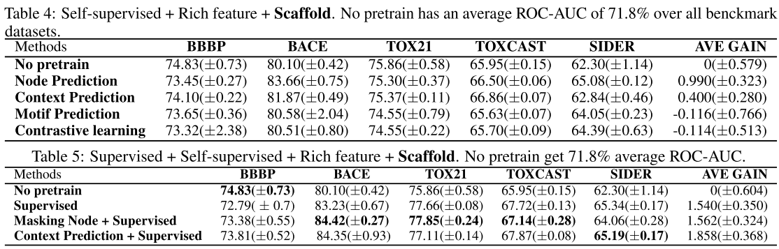
The following table lists the result of default setting:

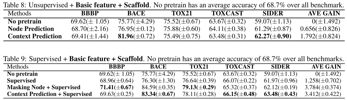
Here is the result of using scaffold data splitting:

Use basic feature:

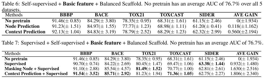
Basic feature + scaffold data splitting:

Main conclusion

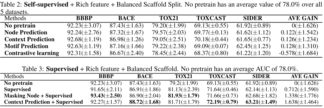
Regardless of the design of the pretraining tasks, applying self-supervised pretraining alone does not provide statistically significant improvements over non-pretrained methods on downstream tasks (from default setting, basic feature, scaffold splitting).
Only when additional supervised pretraining step is conducted after self-supervised pretraining, we might observe statistically significant improvements (from all experiments above).
However, the gain becomes marginal on some specific data splits (from scaffold data splitting) or diminishes if richer features are introduced (compare with basic feature and rich feature).
So, pretraining might help when:
- if we can have the supervised pretraining with target labels that are aligned with the downstream tasks
- if the high quality hand-crafted features are absent (the rich features are calculated from the local environment of atoms, so already contain the useful neighborhood info)
- if the downstream train, valid and test dataset distributions are substantially different.

More experiments & results

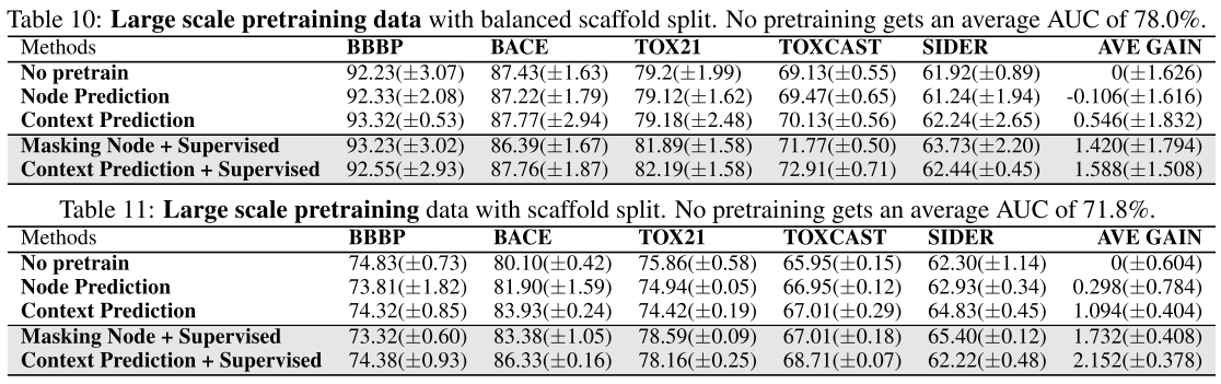
Pretraining on SAVI(larger than ZINC15):

Conclusion:

The SAVI pretraining data does not have a significant improvement either on balanced scaffold split or scaffold split.
Also similarly, the self-supervised pretraining objectives lead to negligible gain on downstream task performance.

Using GraphSAGE architecture:

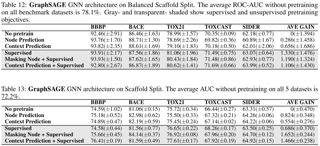
Conclusion:

The conclusion is the same as above. But for larger & deeper GNN it might be different.

Simple reproduce of the original code:

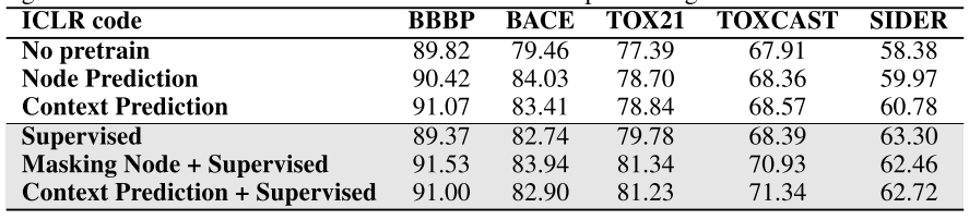
Conclusion:

The usefulness of graph pretraining is also sensitive to the experimental hyperparameters (compared with default)
Suspect the previous success of pretraining may largely due to lack of hyper-parameter tuning and not averaging over different splits.

Pretraining accuracy curve:

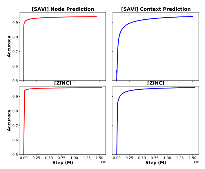
Conclusion:

Tasks are easy: the pre-train task converges fast, which means that some of the self-pretraining tasks for molecules might be easy. So model learns less useful information from pretraining.
The data lacks diversity: molecules share many common sub-structures, e.g., functional motifs. Hence, molecules are not as diversified as text data.
2D Structure is not enough to infer functionality. Some important biophysical properties are barely reflected in the 2D-feature-based pretraining.

Limitations

The study is confined to small molecule graph, so the result can not extend to larger graphs or other fields.
The study focused on representative 1-WL graph neural networks, for architectures go beyond the 1-WL check it might be useful.
And in personal perspective: the SSL tasks might not be designed delicately in the experiment.

Evaluating Self-Supervised Learning for Molecular Graph Embeddings

Model overview

The author designed the following framework for evaluation the graph embedding of different Graph Self-Supervised Learning(GSSL) methods:

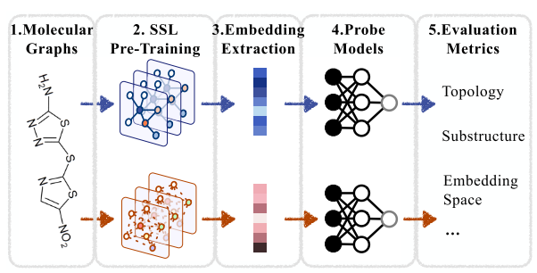
In predicting the evaluation metrics, the GSSL pre-trained backbones are frozen, and only the probe models are trained using extracted node/graph embeddings and corresponding graph metrics.

Experiment settings

GSSL methods for evaluation:

EdgePred: from Inductive representation learning on large graphs.
InfoGraph: from Infograph: Unsupervised and semisupervised graph-level representation learning via mutual information maximization.
GPT-GNN: from Gpt-gnn: Generative pre-training of graph neural networks.
AttrMask & ContextPred: from Strategies for pre-training graph neural networks.
G-Cont & G-Motif: from Self-supervised graph transformer on large-scale molecular data.
GraphCL: from Graph contrastive learning with augmentations.
JOAO: from Graph contrastive learning automated.

Probe models: MLP (should not be too simple or too complex)

Backbone: GIN

Results & conclusions

Performance on downstream tasks

Evaluating GSSL methods on molecular property prediction tasks:

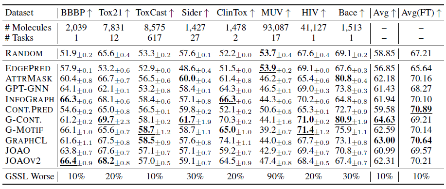
Note that the result in the last two column of the table are result without and with finetuning backbone, respectively.

Conclusions:

Rankings differ among fixed and fine-tuned embeddings.
Random model parameter sometimes beats GSSL methods.

Molecular graph representation evaluation

Generic graph properties
- Node-level statistics: accompany each node with a local topological measure, which could be used as features in node classification
  - Node degree: the number of edges incident to node \(u\), i.e., \(d_u=\sum_{v\in V} A[u,v]\)
  - Node centrality: represents a node’s importance, it is defined as a recurrence relation that is proportional to the average centrality of its neighbours: \(e_u=(\sum_{v\in V}A[u,v]e_v)/\lambda\)
  - clustering coefficient: measures how tightly clustered a node’s neighbourhood is: \(c_u=(|(v_1,v_2)\in E: v_1, v_2\in N(u)|)/d_u^2\). i.e., the proportion of closed triangles in neighbourhood
- Graph-level statistics: summarize global topology information and are helpful for graph classification tasks
  - Diameter: the maximum distance between the pair of vertices.
  - Cycle basis: a set of simple cycles that forms a basis of the graph cycle space. It is a minimal set that allows every even-degree subgraph to be expressed as a symmetric difference of basis cycles.
  - Connectivity: the minimum number of elements (nodes or edges) that need to be removed to separate the remaining nodes into two or more isolated subgraphs.
  - Associativity: measures the similarity of connections in the graph with respect to the node degree. It is essentially the Pearson correlation coefficient of degrees between pairs of linked nodes.
- Pair-level statistics: quantify the relationships between nodes (atoms), which is vital in molecular modelling
  - Link prediction: tests whether two nodes are connected or not, given their embeddings and inner products. Based on the principle of homophily, it is expected that embeddings of connected nodes are more similar compared to disconnected pairs: \(S_{\text{link}}[u,v,x_u^Tx_v^T]=\mathbb{1}_{N(u)}(v)\)
  - Jaccard coefficient: quantify the overlap between neighbourhoods while minimizing the biases induced by node degrees: \(S_{\text{Jaccard}}[u,v]=|N(u)\cap N(v)|/|N(u)\cup N(v)|\)
  - Katz index: a global overlap statistic, defined by the number of paths of all lengths between a pair of nodes: \(S_{\text{Katz}}=\sum_{i=1}^\infty \beta^i A^i[u,v]\)
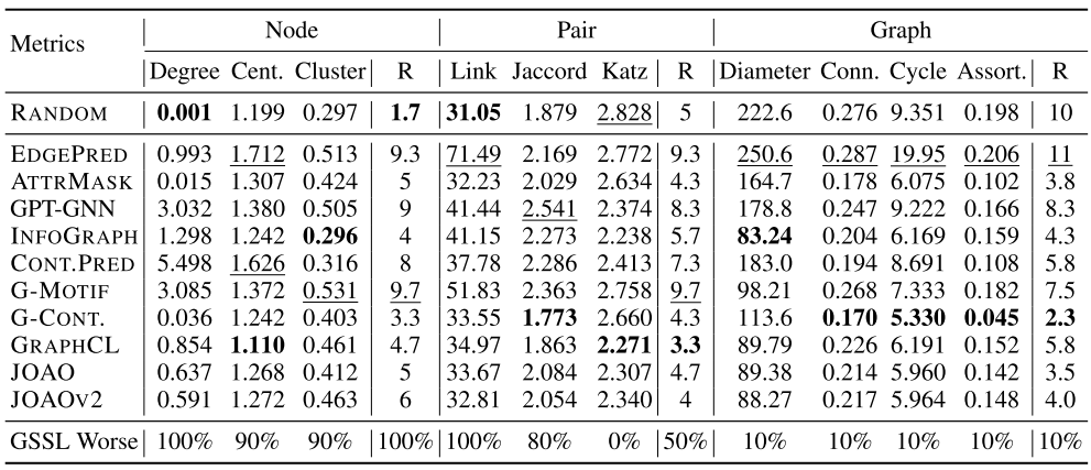
Results:

Conclusion:
- No single method is omnipotent.
- RANDOM outperforms many GSSL methods on node- and pair-level tasks. RANDOM falls short of predicting graph-level metrics.
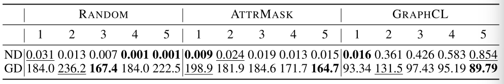
Performance on the topological metrics prediction with embeddings extracted from different layers (Node Degree & Graph Diameter):

Conclusion:
- GSSL learns hierarchical features in a localizable way:
  - The first layer of pre-trained embeddings performs the best on local structural metrics.
  - The last layer of pre-trained embeddings performs the best on global structural metrics.
Molecular substructure properties

Substructure definition: 24 substructures which can be divided into three groups: rings, functional groups, redox Active Sites

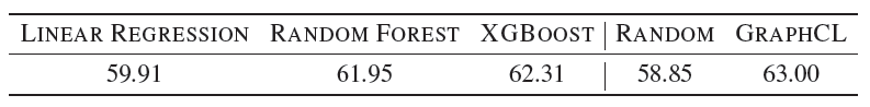
Simply feed counts of substructures within a molecule’s graph into classic ML methods (linear regression, random forest, and XGBoost) to predict the molecule’s properties on eight downstream datasets.

Average scores (same tasks with previous part):

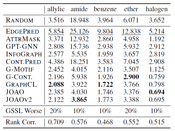
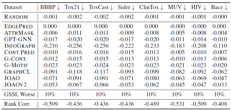
Predict the counts of substructure:

(Rank corr: the Spearman rank correlation between the substructure property and downstream performance)

Conclusions:
- Substructure detection performance correlates well with molecular property prediction performance.
- Contrastive GSSL performs better than in molecular property prediction experiments.
- RANDOM falls short of predicting substructure properties.
Embedding space properties
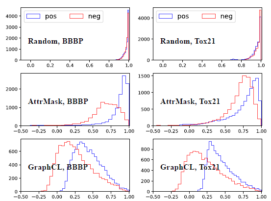
- Alignment: quantifies how similar produced embeddings are for similar samples
  
  The following is the cosine distance histogram of positive and negative pairs:
  
  Conclusion: GSSL methods give rise to better alignment than RANDOM.
- Uniformity: measures how much information is preserved in the embedding space, i.e., how uniformly they are distributed on the unit hypersphere \[ \log \underset{\langle x, y\rangle \sim p_{\text {data }}}{\mathbb{E}}\left[e^{-t\|f(x)-f(y)\|_{2}^{2}}\right], \quad t>0 \]
  
  Conclusion:
  - Relatively speaking, except for EDGEPRED, all GSSL methods achieve uniformity values that are many times less than RANDOM’s.
  - Uniformity rankings do not correlate perfectly with molecular property prediction rankings.
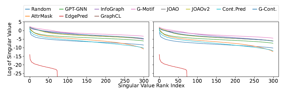
- Dimensional collapse: refers to the problem of embedding vectors spanning a lower-dimensional subspace instead of the entire available embedding space. one simple way to test the occurrence of dimension collapse is to inspect the number of non-zero singular values of a matrix stacking the embedding vectors \(Z=\{z_i\}_{i=1}^N\).
  
  Conclusion:
  - Most GSSL methods “lift” the spectrum compared to RANDOM.
  - EDGEPRED indeed suffered from dimensional collapse.