简介
本文汇总了Physics-informed neural networks: A deep learning framework for solving forward and inverse problems involving nonlinear partial differential equations和Physics-informed machine learning这两篇文章中的主要思想。
在物理学、工程学等领域,经常会遇到数据难以获取的或者获取成本过高的情况,但是前沿的机器学习算法,尤其是神经网络,又无法保证小样本条件下的鲁棒性。考虑到一些实际问题通常需要满足某种物理规律或者经验公式,因此一个可行的办法是将这些模型引入到神经网络的训练过程中,作为网络的正则化项,从而将神经网络的输出限制到某个比较小的取值空间内,使用少量的数据也可以训练出一个预测较为准确的神经网络。而反过来说,将这些结构化的信息输入到模型中也相当于是对原始数据的信息增益,这样便使得模型可以接收到更多的信息,从而加速模型的收敛过程。
PINN
Physics-Informed Neural Network(PINN)这一工作是使用神经网络来近似求解PDE。它的思想是将神经网络作为万能函数近似器来使用,这样便可以直接处理非线性问题,而不需要做先验假设以及线性化等操作。此外,由于深度学习框架的自动微分特性,也可以很容易地求出偏微分的值。同时,神经网络的输出会受到偏微分方程的约束,这样便可以通过方程的约束,使得神经网络满足对称性、不变性和守恒律等物理规则。
一个参数化的非线性PDE具有如下的通用表达式: \[ u_t+\mathcal{N}(u;\lambda)=0, x\in \Omega, t\in [0,T] \] 其中,\(u(t,x)\)代表函数表达式,即PDE的解;\(\mathcal{N}(\cdot;\lambda)\)是一个以\(\lambda\)为参数的非线性运算符;\(\Omega\)是\(\mathbb{R}^D\)的一个子集。例如对于一维的Burgers方程\(u_t+\lambda_1 u u_x-\lambda_2 u_{xx}=0\),它对应的\(\mathcal{N}(\cdot;\lambda)\)为\(\mathcal{N}(u;\lambda)=\lambda_1 u u_x-\lambda_2 u_{xx}\),\(\lambda=[\lambda_1, \lambda_2]\)。
针对于这一表达式,有两个独立的问题。第一个问题是给定\(\lambda\),如何去求解\(u\)的近似表达式;而另一个问题则是能够最好的拟合观测数据的参数\(\lambda\)应当如何取值。
以Burgers方程\(u_t+uu_x=vu_{xx}\)为例,它的模型与如迭代过程如下图所示:

应用
根据PDE求近似函数
如果我们已知一个PDE的表达式\(u_t+\mathcal{N}(u)=0, x\in \Omega, t\in [0,T]\),以及一组与这个PDE相关的数据,那么便可以用神经网络来求解这个PDE的近似函数。根据时间的连续与离散,可分成两种不同种类的模型。
连续时间模型
令\(f(t,x)=u_t+\mathcal{N}(u)\),并使用一个输入为\((t,x)\)的神经网络去近似\(u(t,x)\),由此得到的\(f(t,x)\)便为一个PINN。其中,\(f\)的参数与\(u\)完全一致,\(f\)的表达式可以通过对\(u\)的自动微分来构造。
网络的参数可以通过如下的损失函数来学习: \[ MSE=MSE_u+MSE_f \] 其中, \[ \begin{aligned} MSE_u=&\frac{1}{N_u}\sum_{i=1}^{N_u} |u(t_u^i,x_u^i)-u^i|^2 \\ MSE_f=&\frac{1}{N_f}\sum_{i=1}^{N_f} |f(t_f^i,x_f^i)|^2 \end{aligned} \] 上式中的\(\{t_u^i,x_u^i,u^i\}_{i=1}^{N_u}\)代表\(u(t,x)\)的初始条件与边界条件所对应的训练数据,\(N_u\)代表训练数据的数量。\(\{t_f^i,x_f^i\}_{i=1}^{N_f}\)代表方程\(f(t,x)\)的Collocation points,也就是满足\(f(t,x)=0\)这一约束条件的点。
当数据量比较小的时候,作者使用L-BFGS这一优化算法去求解神经网络的参数;而对于较大规模的数据集,作者使用mini-batch的梯度下降方法去求解。此外作者也提到,虽然这两种优化方法都无法从理论上保证收敛到全局最小,但是在实际情况中,如果神经网络的表达能力足够强,PDE具有唯一解,同时\(N_f\)的值也足够大(即足够的训练样本),那么通常可以获得较高的预测精度。
例:薛定谔方程
考虑如下一个复数域上满足周期性边界条件的薛定谔方程: \[ \begin{aligned} & ih_t+\frac{1}{2}h_{xx}+|h|^2h=0, x\in[-5,5],t\in[0,\frac{\pi}{2}]\\ & h(0,x)=2 \text{sech}(x) \\ & h(t,-5)=h(t,5) \\ & h_x(t,-5)=h_x(t,5) \\ \end{aligned} \] 令\(h(t,x)=[u(t,x)~~v(t,x)]\),其中\(u\)代表复数的实部,\(v\)代表复数的虚部。通过\(h\)我们便可以得到\(f(t,x)=ih_t+\frac{1}{2}h_{xx}+|h|^2h\)这一PINN。网络的参数通过优化如下的损失函数来学习: \[ MSE=MSE_0+MSE_b+MSE_f \] 其中, \[ \begin{aligned} MSE_0=&\frac{1}{N_0}\sum_{i=1}^{N_0} |h(0,x_0^i)-h_0^i|^2 \\ MSE_b=&\frac{1}{N_b}\sum_{i=1}^{N_u} (|h^i(t_b^i,-5)-h^i(t_b^i,5)|^2+|h_x^i(t_b^i,-5)-h_x^i(t_b^i,5)|^2) \\ MSE_f=&\frac{1}{N_f}\sum_{i=1}^{N_f} |f(t_f^i,x_f^i)|^2 \end{aligned} \]
作者在薛定谔方程的实验中,取了50个初始点和50个边界点,以及使用Latin Hypercube采样方法得到的20000个能够覆盖样本空间的Collocation points,使用这些数据训练得到了一个时空维度上都较精确的模型:

对于连续时间模型来说,一个重要的限制就是要求有大量的Collocation points作为训练集,这些点为网络在整个时空维度内都加入了PDE的约束条件。
离散时间模型
对于\(q\)阶的龙格-库塔法求解微分方程,有如下表达式: \[ \begin{aligned} u^{n+c_i}&=u^n-\Delta t\sum_{j=1}^{q}a_{ij}\mathcal{N}[u^{n+c_j}],~~ i=1,\dots,q \\ u^{n+1}&=u^n-\Delta t\sum_{j=1}^{q}b_{j}\mathcal{N}[u^{n+c_j}] \\ \end{aligned} \] 其中,\(u^{n+c_j}(x)=u(t^n+c_j\Delta t,x),j=1,\dots,q\)。上述的通用表达式中,通过选取不同的参数\(\{a_{ij},b_j,c_j\}\),可使得表达式对应于显式和隐式的两种计算方法。
上式也可以写成如下更加简洁的形式: \[ \begin{aligned} &u^n=u_i^n,~~u_i^n=u^{n+c_i}+\Delta t\sum_{j=1}^{q}a_{ij}\mathcal{N}[u^{n+c_j}],~~ i=1,\dots,q \\ &u^n=u_{q+1}^n,~~u_{q+1}^{n}=u^{n+1}+\Delta t\sum_{j=1}^{q}b_{j}\mathcal{N}[u^{n+c_j}] \\ \end{aligned} \] 对于上述的微分方程,可以构造一个输入为\(x\)的PINN,网络的输出为\([u_1^{n}(x),\dots,u_q^{n}(x),u_{q+1}^{n}(x)]\)。
例:Allen-Cahn方程
Allen-Cahn方程用于描述一个反应-扩散系统,例如在一个合金体系中的相分离过程。考虑如下的周期性边界条件PDE: \[ \begin{aligned} &u_t-0.0001u_{xx}+5u^3-5u=0,~~x\in[-1,1],t\in[0,1] \\ &u(0,x)=x^2\cos(\pi x) \\ &u(t,-1)=u(t,1) \\ &u_x(t,-1)=u_x(t,1) \\ \end{aligned} \] 这一PDE对应于\(\mathcal{N}[u^{n+c_j}]=-0.0001u_{xx}^{n+c_j}+5(u^{n+c_j})^3-5u^{n+c_j}\)。
对于上述PDE,可以通过最小化\(SSE=SSE_{n}+SSE_{b}\)来求解网络参数: \[ \begin{aligned} &SSE_n=\sum_{j=1}^{q+1}\sum_{i=1}^{N_n}|u_j^n(x^{n,i})-u^{n,i}|^2 \\ &SSE_b=\sum_{i=1}^{q}|u^{n+c_i}(-1)-u^{n+c_i}(1)|^2+|u^{n+1}(-1)-u^{n+1}(1)|^2+\sum_{i=1}^{q}|u_x^{n+c_i}(-1)-u_x^{n+c_i}(1)|^2+|u_x^{n+1}(-1)-u_x^{n+1}(1)|^2 \end{aligned} \] 其中\(\{x^{n,i},u^{n,i}\}_{i=1}^{N_n}\)代表时间步长为\(t^n\)时的数据。在传统的数值分析算法中,由于稳定性的限制和计算复杂度的限制,时间步长通常会取的很小,因此要计算到所需的时间则需要迭代计算很多步。但是PINN与传统方法相比,则可以在计算代价很小的情况下取一个比较大的阶数\(q\),这样便可以在保证稳定性与精度的前提下取一个较大的时间步长。
在作者的实验中,取该PDE在\(t=0.1\)时刻的200个精确解,作为训练集。然后将时间步长设置为0.8,龙格-库塔法的阶数设为100,对模型进行训练,便得到了精度较高的模型,如下图所示:

求解PDE
连续时间模型
对于参数\(\lambda\)未知的PDE \[ u_t+\mathcal{N}(u;\lambda)=0 \] PINN的求解思路与\(\lambda\)已知的PDE求法类似,同样是构造方程 \[ f=u_t+\mathcal{N}(u;\lambda) \] 其中\(u\)是一个神经网络。此时\(\lambda\)为参数,在求解过程中将会与\(u\)的参数被一同优化。
示例:Naiver-Stokes方程
Naiver-Stokes方程用于描述不可压缩流体的性质。对于一个二维的N-S方程,它的表达式为: \[ u_t+\lambda_1(u u_x+v u_y)=-p_x +\lambda_2(u_{xx}+u_{yy}) \\ v_t+\lambda_1(u v_x+v v_y)=-p_y +\lambda_2(v_{xx}+v_{yy}) \\ \] 其中,\(u(t,x,y)\)代表流速场的\(x\)分量,\(v(t,x,y)\)代表流速场的\(y\)分量,\(p(t,x,y)\)代表压强,\(\lambda=(\lambda_1,\lambda_2)\)为两个未知参数。由于假设流体不可压缩,需要满足流体的质量守恒条件,故N-S方程的解可以在散度为0的方程集合中搜索,即方程的解要满足条件 \[ u_x+v_y=0 \] 故我们可以假设有一个方程\(\psi(t,x,y)\),满足\(u=\psi_y\),\(v=\psi_x\),直接近似求解\(\psi\)便可以自动满足散度为0的约束条件。因此,我们的目标是用一个包含2个输出的神经网络,来同时预测\([\psi(t,x,y),~p(t,x,y)]\)。我们定义 \[ \begin{aligned} f=&u_t+\lambda_1(u u_x+v u_y)+p_x-\lambda_2(u_{xx}+u_{yy})\\ g=&v_t+\lambda_1(u v_x+v v_y)+p_y-\lambda_2(v_{xx}+v_{yy})\\ \end{aligned} \] 从而便可得到一个PINN \([f(t,x,y),~g(t,x,y)]\)。给定一组数据集\(\{t^i,x^i,y^i,u^i,v^i\}_{i=1}^N\),通过最小化如下的损失函数来优化参数\(\lambda\)和神经网络模型的参数: \[ MSE=\frac{1}{N}\sum_{i=1}^{N}\left(|u(t^i,x^i,y^i)-u^i|^2+|v(t^i,x^i,y^i)-v^i|^2 \right)+\frac{1}{N}\sum_{i=1}^{N}\left(|f(t^i,x^i,y^i)|^2+|g(t^i,x^i,y^i)|^2 \right) \] 在作者的实验中,只使用了1%的数据来训练模型,便可得到预测精度较高的\(\lambda\)值。下图为作者对原始数据进行采样的示意图:

当数据没有噪声时,对\(\lambda_1\)和\(\lambda_2\)的预测误差分别为0.078%和4.67%;而对数据加入了1%的高斯噪声之后,模型仍然具有较好的鲁棒性,预测误差分别为0.17%和5.70%。
此外,作者也提到,即使训练数据中并不包含任何关于压力的信息,模型仍然可以预测出较为准确的压力值,如下图所示。图中的数值尺度不一样是因为N-S方程自身的特性决定的,但是图中可以看出它们的数值分布规律基本类似。

离散时间模型
对于\(q\)阶的龙格-库塔法求解微分方程,考虑PDE参数不确定的情况,有如下表达式: \[ \begin{aligned} u^{n+c_i}&=u^n-\Delta t\sum_{j=1}^{q}a_{ij}\mathcal{N}[u^{n+c_j};\lambda],~~ i=1,\dots,q \\ u^{n+1}&=u^n-\Delta t\sum_{j=1}^{q}b_{j}\mathcal{N}[u^{n+c_j},\lambda] \\ \end{aligned} \] 其中,\(u^{n+c_j}(x)=u(t^n+c_j\Delta t,x),j=1,\dots,q\)。上述的通用表达式中,通过选取不同的参数\(\{a_{ij},b_j,c_j\}\),可使得表达式对应于显式和隐式的两种计算方法。
上式也可以写成如下更加简洁的形式: \[ \begin{aligned} &u^n=u_i^n,~~u_i^n=u^{n+c_i}+\Delta t\sum_{j=1}^{q}a_{ij}\mathcal{N}[u^{n+c_j};\lambda],~~ i=1,\dots,q \\ &u^{n+1}=u_{i}^{n+1},~~u_{i}^{n+1}=u^{n+c_i}+\Delta t\sum_{j=1}^{q}(a_{ij}-b_{i})\mathcal{N}[u^{n+c_j};\lambda],~~ i=1,\dots,q \\ \end{aligned} \] 对于上述的微分方程,可以构造一个神经网络去近似\(u\),从而得到两个共享参数的PINN,它们的输出分别为\([u_1^{n}(x),\dots,u_q^{n}(x),u_{q+1}^{n}(x)]\)和\([u_1^{n+1}(x),\dots,u_q^{n+1}(x),u_{q+1}^{n+1}(x)]\)。
如果已知\(n\)时刻和\(n+1\)时刻的一系列采样点\(\{\boldsymbol{x}^n,\boldsymbol{u}^n\}=\{x^{n,i},u^{n,i}\}_{i=1}^{N_n}\)和\(\{\boldsymbol{x}^{n+1},\boldsymbol{u}^{n+1}\}=\{x^{n+1,i},u^{n+1,i}\}_{i=1}^{N_{n+1}}\),便可以使用如下的损失函数对两个网络的参数和PDE的参数\(\lambda\)进行同时优化: \[ SSE=SSE_n+SSE_{n+1} \] 其中, \[ \begin{aligned} &SSE_n=\sum_{j=1}^{q}\sum_{i=1}^{N_n}|u_j^n(x^{n,i})-u^{n,i}|^2 \\ &SSE_{n+1}=\sum_{j=1}^{q}\sum_{i=1}^{N_{n+1}}|u_j^{n+1}(x^{n+1,i})-u^{n+1,i}|^2 \end{aligned} \] 相比于已知参数的PDE,如果\(\lambda\)未知的情况下,对于PDE的约束条件便无法加入到网络中。此时,通过使用时间步长为\(n\)和\(n+1\)时刻的数据,便可以依据PDE的时间关系,从而帮助求解其中的参数\(\lambda\)。
示例:
以浅水表面的水波为例,它满足Korteweg-de Vries(KdV)方程,这一方程描述了一维波的演化过程,例如晶体中的声波、密度分层的海水波等。它的表达式如下: \[ u_t+\lambda_1 uu_x+\lambda_2 u_{xxx}=0 \] 因此对于KdV方程来说,\(\mathcal{N}[u^{n+c_j};\lambda]\)的表达式为 \[ \mathcal{N}[u^{n+c_j};\lambda]=\lambda_1 u^{n+c_j}u_x^{n+c_j}+\lambda_2 u_{xxx}^{n+c_j} \] 在作者的示例中,取连续方程\(u(0,x)=\cos(\pi x)\)作为初始条件,边界满足周期性边界条件,然后进行数值计算得到一系列PDE的离散解。之后,取\(t^n=0.2\)和\(t^{n+1}=0.8\),并在这两个时刻分别采样得到199和201个样本点。使用这些样本点拟合出来的参数与真实值的误差不大于0.1%,如下图所示:

程序示例
示例1:一维热传导方程
一维热传导方程的PDE表达式为: \[ \frac{\partial u}{\partial t}+\frac{\partial^2 u}{\partial x^2}=0, (x)\in [0,1] \] s.t. \[ \begin{aligned} u(x,t)|_{t=0}=&\sin(\pi x) \\ \frac{\partial u(x,t)}{\partial x}|_{x=0}=&\pi \exp(-k\pi^2 t) \\ \frac{\partial u(x,t)}{\partial x}|_{x=1}=&-\pi \exp(-k\pi^2 t) \\ \end{aligned} \] 方程的解析解为: \[ u(x,t)=\sin(\pi {x})\exp(-{k\pi^2 t}) \]
1 | import os |
1 | pi=3.14159265 |
1 | k=0.01 |
1 | t_max=3.0 |
1 | true_values_inner=func(sample_points_inner[:,0],sample_points_inner[:,1]).reshape(-1,1) |
1 | class mlp(nn.Module): |
1 | pinn=mlp().to('cuda') |
1 | pinn.train() |
1 | def plot_contourf(t,x,z): |
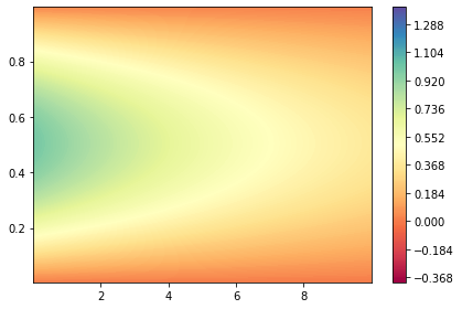
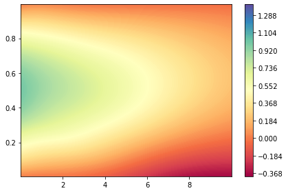
为了验证拟合出的PINN的泛化能力如何,在作图的时候我们取\(t\in [0,10]\),而在训练数据中\(t\)的取值范围仅为\(t\in [0,3]\)。
1 | dt, dx = 0.01, 0.01 |
1 | true_val=func(t.reshape(-1,1),x.reshape(-1,1)) |
1 | pinn.eval() |
从近似值和真实值的分布可以看出,在训练数据的区间内,PINN的拟合效果很好。但是在训练数据的区间之外,拟合效果却不是很好。
1 | plot_contourf(t.reshape(mesh_shape),x.reshape(mesh_shape),true_val.reshape(mesh_shape)) |
1 | plot_contourf(t.reshape(mesh_shape),x.reshape(mesh_shape),pred_val.detach().numpy().reshape(mesh_shape)) |
示例2:拉普拉斯方程
在PINN中举例的PDE都具有\(u_t+\mathcal{N}(u;\lambda)=0, x\in \Omega, t\in [0,T]\)的通用形式,但是对于不带有\(u_t\)项的PDE也可以采用相同的思路,使用神经网络求近似解。
我们以如下的拉普拉斯方程为例,来构造神经网络去近似拟合: \[ \frac{\partial^2 u}{\partial x^2}+\frac{\partial^2 u}{\partial y^2}=0, (x,y)\in [0,1]\times[0,1] \] s.t. \[ \begin{aligned} & u(x,y)|_{x=0}=sin(\pi y) \\ & u(x,y)|_{x=1}=0 \\ & u(x,y)|_{y=0}=0 \\ & u(x,y)|_{y=1}=0 \\ \end{aligned} \]
该PDE的解析解为 \[ u(x,y)=\frac{sin(\pi y)sinh (\pi(1-x))}{sinh (\pi)} \]
1 | import os |
1 | pi=3.14159265 |
1 | def func(x,y): |
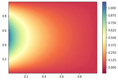
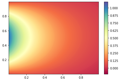
经多次尝试,对于拉普拉斯方程来说,需要在PDE的边界处采样更多的样本点,才能使得最终的拟合效果较好。
1 | sample_points_inner=np.random.uniform(low=0.0,high=1.0,size=(2000,2)) |
1 | true_values_inner=func(sample_points_inner[:,0],sample_points_inner[:,1]).reshape(-1,1) |
1 | class mlp(nn.Module): |
1 | pinn=mlp().to('cuda') |
PINN在训练时波动较大,不太容易训练,因此需要将学习率调得较低一些,并同时使用指数衰减的学习率。
1 | pinn.train() |
1 | dx, dy = 0.01, 0.01 |
1 | true_val=func(x.reshape(-1,1),y.reshape(-1,1)) |
1 | pinn.eval() |
1 | def plot_contourf(x,y,z): |
下图为根据原函数的真实值和PINN的预测值所做出的图像。从中可以看出,二者还是比较接近的。
1 | plot_contourf(x.reshape(mesh_shape),y.reshape(mesh_shape),true_val.reshape(mesh_shape)) |
1 | plot_contourf(x.reshape(mesh_shape),y.reshape(mesh_shape),pred_val.detach().numpy().reshape(mesh_shape)) |
总结
PINN是一种在神经网络的训练过程中引入领域知识的方法,通过将PDE的约束加入到损失函数中,从而可以利用有限数据,使得网络所对应的函数表达式能够尽可能地接近PDE原函数所对应的曲面。同时,这种方法只需要知道PDE的约束条件,而无需任何的额外数据。
在SchNet中将原子力的信息加入到损失函数的方法的思路其实也相当于是加入物理领域知识的额外约束,但是这种方法却需要传入额外的数据(即力的真实值)。因此它与PINN的思路相似,就是将领域知识引入网络的训练过程作为额外约束,但是二者所使用的方法并不相同。总的来说,从这两种方法其实可以得到一种较为通用的思路,即在神经网络的训练中设法引入领域知识。